How Machines Can Learn Using TensorFlow or PyTorch
How Machines Can Learn Using TensorFlow or PyTorch
A deep dive into their minds, their evolution

AI and machine learning are very hot topics these days. Self-driving cars, real-time automatic translation, voice recognition, etc. These are only some of the applications that cannot exist without machine learning. But how can machines learn? I will show you how the magic works in this article, but I won’t talk about neural networks! I will show you what is in the deepest deep of machine learning.
One of the best presentations about machine learning is Fei Fei Li’s TED talk.
As Li said in her talk, in the early days, programmers tried to solve computer vision tasks by algorithms. These algorithms were looking for shapes and tried to identify things by preprogrammed rules. But they could not solve it in this way. Computer vision is a very complex problem, and we cannot solve it algorithmically. So, here comes machine learning into the picture.
If we cannot write the program, let’s write a program that writes it instead of us.
Machine learning algorithms do this. If we have enough data, they can write the algorithm that calculates the expected output from the inputs for us. In the case of image recognition, the input is the image, and the output is a label or a description of the content of the image.
This is why Li and her team worked really hard to build ImageNet, which was the biggest labeled image database in the world, with 15 million images and 22,000 categories.
Thanks to ImageNet, we had enough data, but how did programmers use it to solve the problem of image recognition? This is the point where I should talk about neural networks like Li does, but I won’t. Neural networks are indeed inspired by the biological brain, but today’s transformers are far from the biological model.
This is why I think the name ‘neural network’ is misleading. But what would be a better name?
My favorite is Karpathy’s (head of AI @ Tesla) Software 2.0.
As Karpathy said in this talk, Software 1.0 is the classical software, where the programmer writes the code, but in the case of Software 2.0, another software finds it based on the big data. But how can a software write another software? Let me quote Karpathy:
“Gradient descent can write code better than you. I’m sorry.”
Gradient descent is the name of the magic that is used by most machine learning systems. To understand it, let’s imagine a machine learning system. It’s a black box with inputs and outputs. If the purpose of the system is image recognition, then the input is an array of pixels, and the output is a probability distribution vector.
If the system can identify cats and dogs, and the input is an image of a cat, the output will be like 10% dog and 90% cat. So, the inputs are numbers, the outputs are also numbers, and the content of the black box is a giant (really huge) mathematical expression. The black box calculates the output vector from the pixel data.
I promised to talk about programs writing programs, and now I’m talking about mathematical expression. But in fact, programs are mathematical expressions. CPUs are built from logic gates. They use the binary representation of numbers and logic operators.
Any existing algorithm can be implemented by these logical expressions, so a long logical expression can represent any program that can run on classical computers. As you see, classical programs are also not more than binary calculations from a binary input to a binary output.
Machine learning systems use real numbers and operators instead of binary numbers and operators, but basically, these mathematical expressions are also “programs.”
Alan Turing wrote a paper in 1948 about “B-type unorganized machines.” These machines are built from interconnected logical NAND gates, and can be trained by enabling/disabling the wires between the nodes. In binary algebra, NAND is a universal operator, because every other operator can be expressed by it. These B-type unorganized machines are universal computers because every algorithm can be implemented on them.
These B-type machines are similar to nowadays neural networks, but they are implemented upon logic gates like today’s CPUs, so the algorithms that are implemented by these B-type machines would be more like our today’s algorithms.
Unfortunately, Turing never published the paper, this is why we do not know him as an inventor of early neural networks. The problem with these B-type networks is that they cannot be trained efficiently.
If we have a set of inputs and outputs and a parameterized expression, how can we find the correct parameters that calculate the outputs from the inputs with the fewest error? It is something like a black box that has many potentiometers. Every combination of the potentiometer positions is a program, and we are searching for the correct positions.

To solve this problem, let’s imagine the error function. It looks like a landscape with hills and valleys. Every single parameter of the expression is a dimension of the landscape, and the height of the current point is the error with the given parameters.
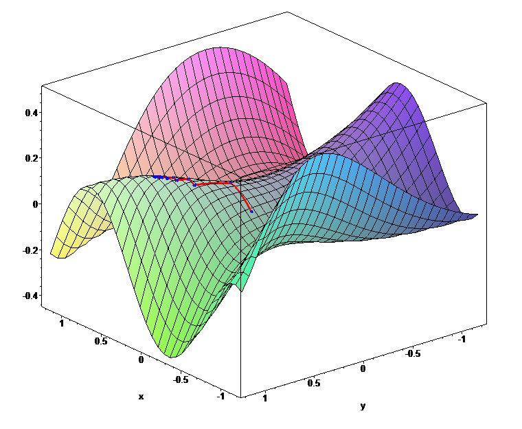
When we initialize the expression with random numbers, we are at a random location on the landscape. To minimize the errors, we have to come down to the lowest point (that represents the lowest error). The problem is that we are completely blind. How can we come down from the hill?
We can grope around to find the steepest slope and go there. But how can we determine the slope of a function? Here comes the gradient in the picture. Gradient shows how steep the slope on the function is at a given point. This is why we call this method “gradient descent.”

The gradient at the given point can be calculated by partial derivation. A function has to satisfy some requirements to be derivable. If we want to use gradient descent for optimization, we have to use these types of functions. If the functions are derivable, then the chain of functions will also be derivable, and there is an algorithmic method to calculate the gradient.
Now we have all the knowledge to understand how TensorFlow and PyTorch (the two most popular machine learning frameworks) find the correct parameters for our expression.
First, let’s look at TensorFlow.
In Tensorflow, there is a gradient registry where gradient functions are registered for the operators by the RegisterGradient method. In the learning phase, in every step, a GradientTape has to be started. GradientTape is something like a video recorder. When TensorFlow does any operation, the gradient tape logs it.
After the end of the forward phase (when the output is generated from the input), we stop the gradient tape that goes backward on the log by using the error and calculating the gradients using the registered gradient functions. We can modify the parameters and repeat the process until we reach the minimum error by using the gradients.
Let’s look at the code in Python:
This code shows how we can solve the simplest problem (linear regression) by using gradient descent in TensorFlow. The aim of linear regression is to find the parameters of a line that is closest to each point, where closest means that the sum of squares of the distances is minimal.
TensorFlow uses tensor operations for the calculations. Tensors are generalizations of matrices. From the programmer’s perspective, tensors are simple arrays. A zero-dimensional tensor is a scalar, a one-dimensional tensor is a vector, a two-dimensional tensor is a matrix, and from third dimension, tensors are simply tensors. Tensor operations can be done in parallel to run efficiently, especially on GPUs or TPUs.
At the beginning of the code, we define our model, which is a linear expression. It has two scalar parameters, W and b, and the expression is y=W*x+b. The default value of W is 16, and b is 10. This is in our black box, our code will change the W and the b to minimize the error. Real-world models have millions or billions of parameters, but these two parameters are enough to understand the method.
From line 21 to line 23, we define the random point set. The tf.random.normal method generates a vector with 1,000 random numbers in a normal distribution, and we use that to generate the points near a line.
The loss function is defined in line 34. y and y_pred parameters are vectors. y_pred is the actual output of our model, and y is the expected output. The square function calculates the square of every vector element, and the output is also a vector with the squares. The reduce_mean function calculates the mean of elements, and its result is a scalar. This is the error itself that we want to minimize.
The gradient descent is from line 36 to line 42. This is the essence of the code where the learning happens. The with in line 37 is a Python expression. It calls the parameter object’s __enter__ method at the beginning of the block and __exit__ at the end.
In the case of GradientTape, the __enter__ method starts the recording, and __exit__ stops it. In the block (line 38), we calculate the model output by model(X) and the error. In line 40, the GradientTape calculates the gradients for the parameters (dW and db), and in lines 41 and 42, modify the parameters.
There are different optimization strategies. We are using the simplest, where the gradients are multiplied by a fixed learning rate (lr).
In a nutshell, this is how gradient descent and TensorFlow’s GradientTape work. You can find many tutorials on TensorFlow’s webpage. Neural networks for image recognition, reinforcement learning, etc., but keep in your mind, there are always tensor operations and a GradientTape.
Now, let’s see how gradient descent works in the other big framework, PyTorch.
PyTorch uses the autograd system for gradient calculation, which is embedded into the torch tensors. If a tensor is a result of an operator, it contains a back pointer to the operator and the source tensors. The source tensors also contain back pointers, etc., and the full operator chain is traceable.
Every operator can calculate its own gradient. When you call the backward method on the last tensor, it goes back on the chain and calculates the gradients to the tensors.
Let’s see the previous linear regression code in PyTorch:
The model and the loss part are very similar to TensorFlow. You find the difference in the train method from line 37 to line 46. After the calculation of the current_loss tensor, we call the backward method on it. It recursively goes back on the chain and calculates the gradient for the W and b tensors.
From line 41 to line 43, we modify the W and b tensors. It’s important that this calculation is in a torch.no_grad() block. The no_grad() method temporarily disables the gradient calculation for the operators, which is not needed when we modify the parameters.
At the end of the train method calling the zero method clears the gradients. Without this, PyTorch will sum up the gradients, which results in strange behavior. The other parts of the code are very similar to TensorFlow. Like TensorFlow, PyTorch also has good tutorials, community, and documentation.
You will find everything to build any neural network, but the most important part is the autograd system, which is the base of the training.
Next time, when you see a picture that DALL-E generates, a car that drives itself, or simply wonder how Google Assistant understands what you say, you will know how the magic works, and how an algorithm (the gradient descent) wrote these cool algorithms for us.